Exploring Google's ortools - Part 1
Introduction to linear programming and optimization with ortools.
Introduction
I recently came across Google's ortools library and I was immediately curious to explore it. I wanted to give it a try against some of the optimization problems I used to solve using a combination of Excel's Solver1 and the Simplex method2 some years ago. I decided to start with a simple linear programming problem and see how it goes.
The problem comes from exercise 3.3 of Linear Programming and Network Flows3.
Consider the following problem:
Solution
Graphical Solution
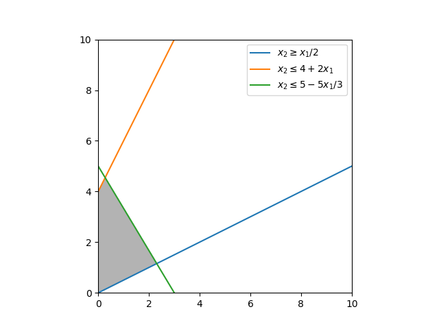
The graphical solution is straightforward. We plot the constraints and find the feasible region. Then we plot the objective function and find the optimal solution.
from functools import reduce
from operator import and_

import matplotlib.pyplot as plt
import numpy as np

d = np.linspace(0, 10, 300)
x, y = np.meshgrid(d, d)

# Create conditions for the feasible region
conditions = (
    (x >= 0),
    (y >= 0),
    (x - 2 * y <= 0),
    (-2 * x + y <= 4),
    (5 * x + 3 * y <= 15),
)

# Plot the feasible region
plt.imshow(
    reduce(and_, conditions),  # apply & operator to all conditions
    extent=(x.min(), x.max(), y.min(), y.max()),
    origin="lower",
    cmap="Greys",
    alpha=0.3,
)

# Plot the constraints
x = np.linspace(0, 16, 2000)
c1_y = x / 2
c2_y = 4 + 2 * x
c3_y = (15 - 5 * x) / 3

plt.plot(x, c1_y, label=r"$x_2 \geq x_1/2$")
plt.plot(x, c2_y, label=r"$x_2 \leq 4 + 2x_1$")
plt.plot(x, c3_y, label=r"$x_2 \leq 5 - 5x_1/3$")
plt.xlim(0, 10)
plt.ylim(0, 10)

plt.legend()
plt.savefig("../../posts/img/ortools/ex3_3_graphical_solution.png")
Output
The feasible region is the shaded area in the plot below.
Analysis
From the plot, we can see that the optimal solution is at the intersection of the lines \(x_2 = 4 + 2x_1\) and \(x_2 = 5 - 5x_1/3\). The optimal solution is at \(x_1 = \frac{3}{11}\) and \(x_2 = \frac{50}{11}\), and the optimal value of the objective function is \(\frac{153}{11} \approx 13.91\).
Solution with ortools
Now, let's solve the same problem using ortools.
"""Solve exercise 3.3 from the book.

Maximize      X1 + 3X2
subject to    X1 - 2X2 <= 0
            -2X1 +  X2 <= 4
             5X1 + 3X2 <= 15
              X1,   X2 >= 0.
"""

import sys

from ortools.linear_solver import pywraplp

# Create the linear solver with the GLOP backend
solver = pywraplp.Solver.CreateSolver("GLOP")
if not solver:
    print("The solver could not be created.")
    sys.exit(1)

# Create the variables x and y.
x1 = solver.NumVar(0, solver.infinity(), "x1")
x2 = solver.NumVar(0, solver.infinity(), "x2")
print("Number of variables =", solver.NumVariables())

# Create a linear constraint, X1 - 2X2 <= 0.
ct = solver.Constraint(-solver.infinity(), 0, "ct0")
ct.SetCoefficient(x1, 1)
ct.SetCoefficient(x2, -2)

# Create a linear constraint, -2X1 + X2 <= 4.
ct = solver.Constraint(-solver.infinity(), 4, "ct1")
ct.SetCoefficient(x1, -2)
ct.SetCoefficient(x2, 1)

# Create a linear constraint, 5X1 + 3X2 <= 15.
ct = solver.Constraint(-solver.infinity(), 15, "ct2")
ct.SetCoefficient(x1, 5)
ct.SetCoefficient(x2, 3)

print("Number of constraints =", solver.NumConstraints())

# Create the objective function, X1 + 3X2.
objective = solver.Objective()
objective.SetCoefficient(x1, 1)
objective.SetCoefficient(x2, 3)
objective.SetMaximization()

print(f"Solving with {solver.SolverVersion()}")
status = solver.Solve()

if status == pywraplp.Solver.OPTIMAL:
    print("Solution:")
    print("Objective value =", objective.Value())
    print("X1 =", x1.solution_value())
    print("X2 =", x2.solution_value())
else:
    print("The problem does not have an optimal solution.")

print("\nAdvanced usage:")
print(f"Problem solved in {solver.wall_time():d} milliseconds")
print(f"Problem solved in {solver.iterations():d} iterations")
Output
The output of the script is:
Number of variables = 2
Number of constraints = 3
Solving with Glop solver v9.9.3963
Solution:
Objective value = 13.909090909090907
X1 = 0.2727272727272725
X2 = 4.545454545454545

Advanced usage:
Problem solved in 0 milliseconds
Problem solved in 2 iterations
Conclusion
As you can see, ortools reached the same optimal solution as the graphical solution. The library is easy to use and provides a simple interface to solve optimization problems.
In this blog post we explored a simple linear programming problem, but ortools can also solve other types of optimization problems, including:
- Constraint optimization
- Mixed-integer optimization
- Assignment
- Scheduling
- Packing
- Routing
- Network flows
In the next post, we will explore a different type of optimization problem using ortools.
Appendix: environment
The following lock file was used to set up the environment for running the scripts.
# This file was autogenerated by uv via the following command:
#    uv pip compile --output-file=requirements.txt requirements.in
absl-py==2.1.0
    # via ortools
contourpy==1.2.0
    # via matplotlib
cycler==0.12.1
    # via matplotlib
fonttools==4.50.0
    # via matplotlib
immutabledict==4.2.0
    # via ortools
kiwisolver==1.4.5
    # via matplotlib
matplotlib==3.8.3
    # via -r requirements.in
numpy==1.26.4
    # via
    #   -r requirements.in
    #   contourpy
    #   matplotlib
    #   ortools
    #   pandas
ortools==9.9.3963
    # via -r requirements.in
packaging==24.0
    # via matplotlib
pandas==2.2.1
    # via ortools
pillow==10.3.0
    # via matplotlib
protobuf==5.26.1
    # via ortools
pyparsing==3.1.2
    # via matplotlib
python-dateutil==2.9.0.post0
    # via
    #   matplotlib
    #   pandas
pytz==2024.1
    # via pandas
six==1.16.0
    # via python-dateutil
tzdata==2024.1
    # via pandas
-
Solver is a Microsoft Excel add-in program you can use to find an optimal value for the formula in a cell. ↩
-
The Simplex method is a popular algorithm for solving linear programming problems. ↩
-
Mokhtar S. Bazaraa, John J. Jarvis, Hanif D. Sherali, Linear Programming and Network Flows, 4th Edition, Wiley, 2010. ↩